[Deep Learning/딥 러닝] 최적화 기법
- 30분 내 담기에 너무 방대한 주제
- 각각의 분야마다 최소 한 학기 이상 공부하는 분야
- 줄이고 줄여서 실제로 적용 시 중요하게 알아두어야 할 개념들 위주로
Introduction
Gradient Descent
- 1st-order iterative optimization algorithm for finding a local minimum of a differentiable function.
Important Concepts in Optimization
- Generalization
- Underfitting vs. overfitting
- Cross-validation
- Bias-variance trade-off
- Bootstrapping
- Bagging and boosting
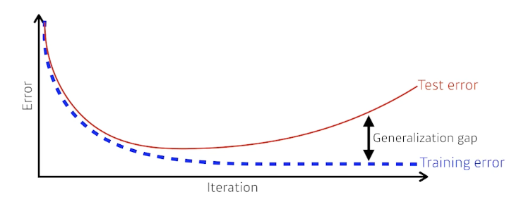
Generalization
- How well the learned model will behave on unseen data.
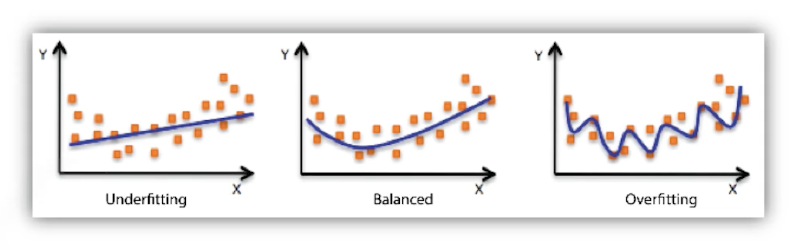
Underfitting vs. Overfitting
Cross-validation
- Cross-validation is a model validation technique for assessing how the model will generalize to an independent (test) dataset.
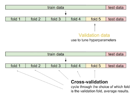
- CV를 통해서 최적의 hyperparameter set을 찾고 hyperparameters를 고정한 상태에서 학습시킬 때는 모든 데이터를 사용 → 더 많은 데이터를 가지고 학습하고자!
- 테스트 데이터셋은 그 어떠한 경우에도 사용 불가 \(\because\) cheating
Bias and Variance
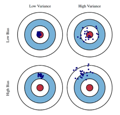
- Variance: 비슷한 입력에 대해 출력이 얼마나 일관적으로 나오는가를 측정
- Bias: 여러 입력에 대한 출력들이 평균적으로 얼마나 true값에 가까운가를 측정
Bias and Variance Trade-off
Given \(\mathcal D=\{(x_i,t_i)\}_{i=1}^N\), where \(t=f(x)+\epsilon\) and \(\epsilon\sim\mathcal N(0,\sigma^2)\).
We can derive that what we are minimizing (cost) can be decomposed into three different parts: bias, variance, and noise. \[\begin{aligned}\underbrace{\mathbb E\left[(t-\hat f)^2\right]}_\text{cost}&=\mathbb E\left[(t-f+f-\hat f)^2\right]\\&=\cdots\\&=\underbrace{\mathbb E\left[\left(f-\mathbb E[\hat f]^2\right)^2\right]}_{\text{bias}^2}+\underbrace{\mathbb E\left[\left(\mathbb E[\hat f]-\hat f\right)^2\right]}_\text{variance}+\underbrace{\mathbb E[\epsilon]}_\text{noise}\end{aligned}\]
- Bias, variance 둘 모두를 줄이는 것이 힘들다는 기본적 제약
Bootstrapping
- Bootstrapping is any test or metric that uses random sampling with replacement.
- 학습 데이터의 일부를 임의로 구성/활용(subsampling)한 모델을 여럿 사용한다고 할 때, 모델들의 예측값들의 consensus를 확인하고 전체 모델의 uncertainty를 확인하고자 하는 기법
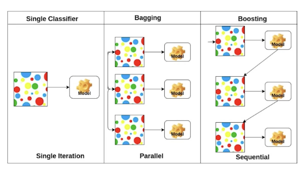
Bagging vs. Boosting
- Bagging (Bootstrapping aggregating)
- Multiple models are being trained with bootstrapping.
- E.g., base classifiers are fitted on random subset where individual predictions are aggregated (voting or averaging).
- 여러 모델의 예측값의 voting이나 평균을 취하는 방식이 단일 모델의 성능보다 좋은 경우가 많음
- Boosting
- It focuses on those specific training samples that are hard to classify.
- A strong model is built by combining weak learners in sequence where each learner learns from the mistakes of the previous weak learner.
- Baseline 모델이 취약한 데이터에 대해서 보완 모델을 만들고, 또 이 모델이 취약한 데이터에 대해 보완 모델을 만들어 sequential하게 모델을 이어 robustness를 키우는 방식
Practical Gradient Descent Methods
Gradient Descent Methods
- Stochastic gradient descent
- Update with the gradient computed from a single sample.
- Mini-batch gradient descent
- Update with the gradient computed form a subset of data.
- Batch gradient descent
- Update with the gradient computed from the whole data.
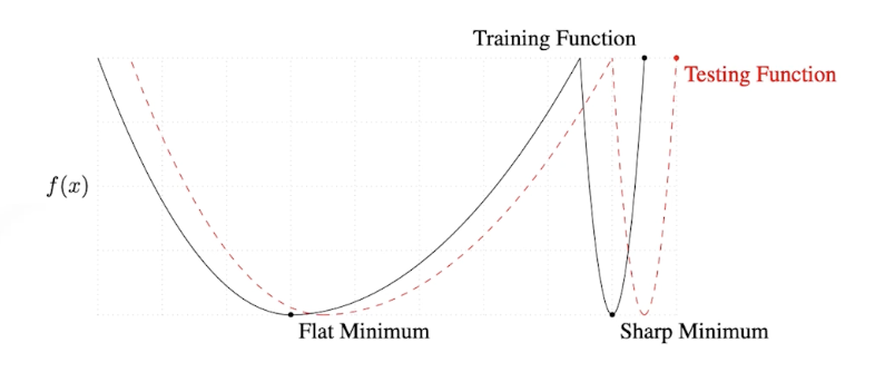
Batch-size matters
- “It has been observed in practice that when using a larger batch there is a degradation in the quality of the model, as measured by its ability to generalize.”
- “We … present numerical evidence that supports the view that large batch methods tend to converge to sharp minimizers of the training and testing functions. In contrast, small-batch methods consistently converge to flat minimizers… this is due to the inherent noise in the gradient estimation.”
- Batch-size를 작게 설정하여 sharp minimizers보다는 flat minimizers에 도달하는 것이 낫다는 이야기
- On Large-batch Training for Deep Learning Generalization Gap and Sharp Minima, 2017. (논문 리딩 추천)
Gradient Descent Methods
- SGD
- Momentum
- Nesterov accelerated gradient
- Adagrad
- Adadelta
- RMSprop
- Adam
(Stochastic) Gradient Descent
\[W_{t+1}\leftarrow W_t-\eta g_t\]- 문제: learning rate (or step size) \(\eta\)를 적절히 잡는 것이 너무 어려움
Momentum
\[\begin{aligned} a_{t+1}&\leftarrow\beta a_t+g_t\\W_{t+1}&\leftarrow W_t-\eta a_{t+1} \end{aligned}\]- 이전의 gradient 방향 정보를 다음 gradient에도 반영하자는 아이디어 — 관성(momentum)
- 해석
- \(\beta\): momentum
- \(a\): accumulation
- 한 번 흘러가기 시작한 gradient path를 어느 정도 유지시켜줌 → mini-batch gradient의 randomness가 있다고 하더라도 학습 효과를 향상 시켜줌.
Nesterov Accelerated Gradient (NAG)
\[\begin{aligned} a_{t+1}&\leftarrow\beta a_t+\nabla\mathcal L(W_t-\eta\beta a_t)\\W_{t+1}&\leftarrow W_t-\eta a_{t+1} \end{aligned}\]- 해석
- \(\nabla\mathcal L(W_t-\eta\beta a_t)\): lookahead gradient
- 가장 큰 장점: 비교적 빠르게 local minima로 수렴
- 이론적으로도 momentum에 비해 높은 converge ratio를 가짐을 증명 가능
- Momentum 방식과 달리, \(a\) 방향으로 이동한 뒤 gradient를 계산하여 이동
Adagrad
\[W_{t+1}\leftarrow W_t-\frac{\eta}{\sqrt{G_t+\epsilon}}g_t\]- Adagrad adapts the learning rate, performing larger updates for infrequent and smaller updates for frequent parameters.
- 신경망의 파라미터가 현재까지 얼마나 변해왔는지, 안 변했는지를 살핌 — 크게 변화해 온 파라미터는 더 적게, 적게 변화해 온 파라미터는 더 크게 변화시키려고 함
- 해석
- \(G_t\): sum of gradient squares
- \(\epsilon\) ~ for numerical stability
- 문제
- \(G_t\)가 지속적으로 커짐에 따라 긴 시간 학습 시 학습이 멈춰지는 현상 발생
- What will happen if the training occurs for a long period?
Adadelta
\[\begin{aligned} G_t&=\gamma G_{t-1}+(1-\gamma)g_t^2\\W_{t+1}&=W_t-\frac{\sqrt{H_{t-1}+\epsilon}}{\sqrt{G_t+\epsilon}}g_t\\H_t&=\gamma H_{t-1}+(1-\gamma)(\Delta W_t)^2 \end{aligned}\]- Adadelta extends Adagrad to reduce its monotonically decreasing the learning rate by restricting the accumulation window.
- Adagrad의 문제를 해결할 쉬운 아이디어: 현재 timestep \(t\)에서 어느 정도 window size만큼 gradient의 제곱의 변화에 얼마나 민감한지 확인
- 하지만 이와 같은 방식은 window size에 따라 이전 정보를 얼마나 보존하고 있어야 하는지가 달라지는데, GPT-3와 같이 \(G_t\)가 1000억 여개 이상의 파라미터 수를 가지는데 이를 수 window size만큼의 배수의 정보를 보존하고 있는 것이 불가능
이를 막을 수 있는 방법?
→ exponential moving average (EMA)
- 특징: learning rate 존재 x → 바꿀 수 있는 부분이 적어 많이 활용하지 않음
- 해석
- \(G_t\): EMA of gradient squares
- \(H_t\): EMA of difference squares
RMSprop
- RMSprop is an unpublished, adaptive learning rate method proposed by Geoffrey Hinton in his lecture.
- 해석
- \(G_t\): EMA of gradient squares
- \(\eta\): step size
Adam
\[\begin{aligned} m_t&=\beta_1m_{t=1}+(1-\beta_1)g_t\\v_t&=\beta_2v_{t-1}+(1-\beta_2)g_t^2\\W_{t+1}&=W_t-\frac{\eta}{\sqrt{v_t+\epsilon}}\frac{\sqrt{1-\beta_2^t}}{1-\beta_1^t}m_t \end{aligned}\]- Adaptive Momenet Estimation (Adam) leverages both past gradients and squared gradients.
- 일반적으로 잘 되고 가장 무난하게 사용하는 방식
- Momentum + adaptive learning rate approach
- 해석
- \(m_t\): momentum
- \(v_t\): EMA of gradient squares
- \(\eta\): step size
- Tip: \(\epsilon=10^{-7}\)을 잘 바꾸어 주는 것이 중요 in practice
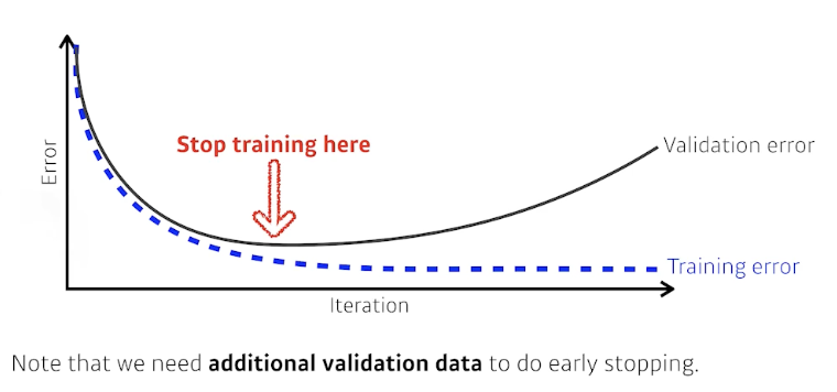
Regularization
- Early stopping
- Parameter norm penalty
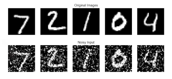
- Data augmentation
- Noise robustness
- Label smoothing
- Dropout
- Batch normalization
Early stopping
Parameter norm penalty
- This adds smoothness to the function space.
- Weight decay라고도 함
- 해석
- 신경망이 만들어내는 function space에서 이 함수를 최대한 부드러운(smooth) 함수로 보자는 것
- Why? 부드러운 함수(smooth function)일수록 일반화 성능(generalization performance)이 좋을 것
Data augmentation
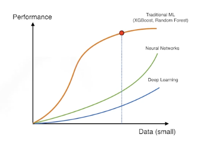
- 데이터가 무한히 많으면, 웬만하면 잘 됨
- 데이터가 적은 경우, 데이터 증대(data augmentation) 필요ㅈ
Noise robustness
- 입력 또는 파라미터에 random noise를 추가하는 것
- 왜 잘 되는가에 대해서는 아직까지 의문이 존재
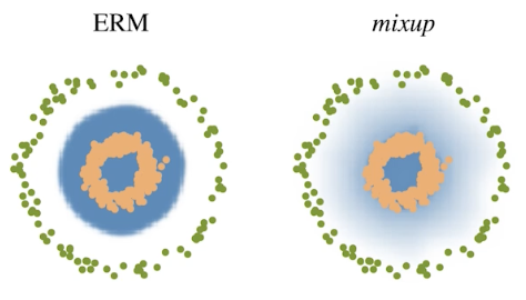
Label smoothing
- Mix-up constructs augmented training examples by mixing both input and output of two randomly selected training data.
- Decision boundary 부드럽게 만들어주는 효과
CutMix constructs augmented training examples by mixing inputs with cut and paste and outputs with soft labels of two randomly selected training data.
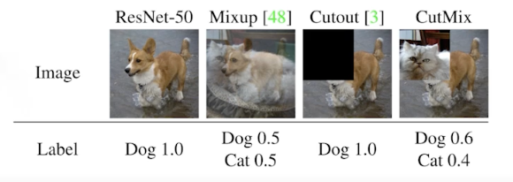
- 성능이 굉장히 많이 올라감!
- 들이는 노력 대비 성능을 많이 올릴 수 있는 방법
Dropout
- In each forward pass, randomly set some neurons to zero.
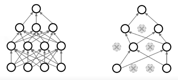
- 해석
- 각각의 neuron들로부터 추출되는 robust features가 남음
- 수학적으로 엄밀히 증명된 것은 아님
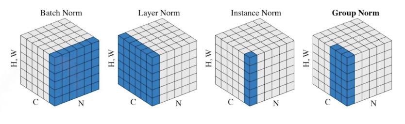
Batch normalization
- Batch normalization compute the empirical mean and variance independently for each dimension (layers) and normalize.
- 논란이 있는 부분: internal covariate shift
- 신경망 층을 많이 쌓을 때 BN을 활용하면 성능이 올라감
- 논문의 해석
- 평균을 0으로, 분산을 1로 만들어줌으로써 internal covariate (feature) shift가 줄어든다
- 이후 논문들은 이에 대해 반박
마무리
- 네트워크를 만들고, 데이터와 문제 등이 고정되어 있을 때, 이러한 정규화(regularization) 기법을 사용해보면서 일반화 성능(generalization performance)을 살핌