[Deep Learning/딥 러닝] 생성 모델
Generative Models Part 1
Introduction
- What does it mean by learning a generative model?
Learning a Generative Model
- Suppose that we are given images of dogs.
- We want to learn a probability distribution \(p(x)\) such that
- Generation: If we sample \(\tilde x\sim p(x)\), \(\tilde x\) should look like a dog.
- Density estimation: \(p(x)\) should be high if \(x\) looks like a dog, and low otherwise.
- This is also known as an explicit models.
- Then how can we represent \(p(x)\)?
Basic Discrete Distributions
- Bernoulli distribution: (biased) coin flip
- Sample space \(D=\{\text{Heads}, \text{Tails}\}\).
- Specify \(P(X=\text{Heads})=p\). Then \(P(X=\text{Tails})=1-p\).
- Say \(X\sim\text{Ber}(p)\).
- Categorical distribution: (biased) \(m\)-sided dice
- Sample space \(D=\{1,\cdots,m\}\).
- Specify \(P(Y=i)=p_i\) such that \(\sum_{i=1}^mp_i=1\).
- Say \(Y\sim\text{Cat}(p_1,\cdots,p_m)\).
Example
- Modeling a single pixel of an RGB image.
- Color tuple \((r,g,b)\sim p(R,G,B)\)
- Number of cases = \(256\times256\times256\)
How many parameters do we need to specify? \[256\times256\times256-1\]
Independence
Example
- Suppose we have \(X_1,\cdots,X_n\) of binary pixels (a binary image).
- Number of cases = \(2^n\)
How many parameters do we need to specify? \[2^n-1\]
→ Almost impossible to model a distribution
Structure through Independence
- Suppose independencies among \(X_i’s\) for \(i=1,\cdots,m\)
- Number of cases = \(2^n\)
- However parameters we need to specify = \(n\).
→ Bad modeling that can represent a meaningful distribution
Conditional Independence
- 위 두 assumptions의 중간 어딘가의 타협점을 찾기 위해..
- Three important rules
Chain rule \[p(x_1,\cdots,x_n)=p(x_1)p(x_2|x_1)p(x_3|x_1,x_2)\cdots p(x_n|x_1,\cdots,x_{n-1})\]
Bayes’ rule \[p(x|y)=\frac{p(x,y)}{p(y)}=\frac{p(y|x)p(x)}{p(y)}\]
Conditional independence
If \(x\perp y\vert z\), then \[p(x|y,z)=p(x,z)\]
Using chain rule we obtain \[P(X_1,\cdots,X_n)=P(X_1)P(X_2|X_1)\cdots P(X_n|X_1,\cdots,X_{n-1})\]
- How many parameters?
- For each term \(P(X_i\vert X_{i-1},\cdots)\), \(2^{i-1}\) parameters needed
- The total sum becomes \(1+2+\cdots+2^{n-1}=2^n-1\).
Now we suppose Markov assumption: \(X_{i+1}\perp X_1,\cdots,X_{i-1}\perp X_i\), then the above equation becomes \[p(x_1,\cdots,x_n)=p(x_1)p(x_2|x_1)p(x_3|x_2)\cdots p(x_n|x_{n-1})\]
How many parameters? \[2n-1\]
- Hence by leveraging the Markov assumption, we get exponential reduction on the number of parameters.
- Autoregressive models leverages this conditional independency.
Autoregressive Models
- Suppose we have \(28\times28\) binary pixels.
- Our goal is to learn \(P(X)=P(X_1,\cdots,X_{784})\) over \(X\in\{0,1\}^{784}\).
- Then how can we parametrize \(P(X)\)?
- Let’s use the chian rule to factor the joint distribution.
An autoregressive model: \[P(X_{1:784})=P(X_1)P(X_2|X_1)P(X_3|X_2)\cdots\]
- Note that we need an ordering (e.g., raster scan order) of all random variables.
NADE: Neural Autoregressive Density Estimator
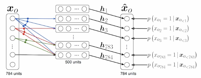
The probability distribution of \(i\)-th pixel is \[p(x_i|x_{1:i-1})=\sigma(\alpha_i\mathbf h_i+b_i)\;\;\text{where}\;\;\mathbf h_i=\sigma(W_{<i}x_{1:i-1}+\mathbf c)\]
- NADE is an explicit model that can compute the density of the given inputs.
- How can we compute the density of the given image?
- Suppose that we have a binary image with 784 binary pixels i.e., \(\{x_1,x_2,\cdots,x_{784}\}\).
Then the joint probability is computed by \[p(x_1,\cdots,x_{784})=p(x_1)\cdots p(x_{784}|x_{1:783})\]
where each conditional probability \(p(x_i\vert x_{1:i-1})\) is computed independently.
- In case of modeling continuous random variables, a mixture of Gaussian (MoG) can be used.
Summary of Autoregressive Models
- Easy to sample from
- Sample \(\tilde x_0\sim p(x_0)\)
- Sample \(\tilde x_1\sim p(x_1\vert x_0=\tilde x_0)\)
- and so forth (in a sequential manner, hence slow).
- Easy to compute probability \(p(x=\tilde x)\)
- Compute \(p(x_0=\tilde x_0)\)
- Compute \(p(x_1=\tilde x_1\vert x_0=\tilde x_0)\)
- Multiply together (sum their logarithms)
- and so on.
- Ideally we can compute all these terms in parallel.
- Easy to be extended to continuous variables. E.g., we can choose mixture of Gaussians.
Generative Models Part 2
Maximum Likelihood Learning
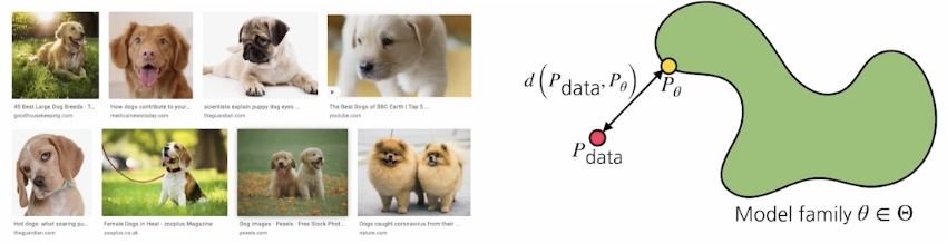
- Given a training set of examples, we can cast the generative model learning process as finding the best-approximating density model from the model family.
- Then how can we evaluate the goodness of the approximation?
KL-divergence ~ symmetric property를 만족하지 않으나 “근사적으로” 두 분포사이의 거리를 의미하는 것으로 해석 \[\begin{aligned}\mathcal D(P_\text{data}\Vert P_\theta)&=\mathbb E_{\mathbf x\sim P_\text{data}}\left[\log\left(\frac{P_\text{data}(\mathbf x)}{P_\theta(\mathbf x)}\right)\right]\\&=\int P_\text{data}(\mathbf x)\log\frac{P_\text{data}(\mathbf x)}{P_\theta(\mathbf x)}\;\text{d}\mathbf x\end{aligned}\]
We can simplify the above as follows: \[\begin{aligned}\mathcal D(P_\text{data}\Vert P_\theta)&=\mathbb E_{\mathbf x\sim P_\text{data}}\left[\log\left(\frac{P_\text{data}(\mathbf x)}{P_\theta(\mathbf x)}\right)\right]\\&=\mathbb E_{\mathbf x\sim P_\text{data}}[\log P_\text{data}(\mathbf x)]-\mathbb E_{\mathbf x\sim P_\text{data}}[\log P_\theta(\mathbf x)]\end{aligned}\]
As the first term does not depend on \(P_\theta\), minimizing the KL-divergence is equivalent to maximizing the expected log-likelihood. \[\begin{aligned}\arg\min_{P_\theta}\mathcal D(P_\text{data}\Vert P_\theta)&=\arg\min_{P_\theta}-\mathbb E_{\mathbf x\sim P_\text{data}}[\log P_\theta(\mathbf x)]\\&=\arg\max_{P_\theta}\mathbb E_{\mathbf x\sim P_\text{data}}[\log P_\theta(\mathbf x)]\end{aligned}\]
Approxmiate the expected log-likelihood \[\mathbb E_{\mathbf x\sim P_\text{data}}\left[\log P_\theta(\mathbf x)\right]\]
with the empirical log-likelihood \[\mathbb E_\mathcal D[\log P_\theta(\mathbf x)]=\frac{1}{|\mathcal D|}\int_{\mathbf x\in\mathcal D}\log P_\theta(\mathbf x)\;\text{d}\mathbf x\]
- 분포 \(P_\text{data}\)을 직접적으로 알 수 없는 상황에서 관측한 데이터셋 \(\mathcal D\)가 분포 \(P_\text{data}\)를 가진다고 가정하고 parametrized distribution을 학습하겠다는 것
Maximum likelihood learning is then \[\max_{P_\theta}\frac{1}{|\mathcal D|}\int_{\mathbf x\in\mathcal D}\log P_\theta(\mathbf x)\;\text{d}\mathbf x\]
Variance of Monte Carlo estimate is high: \[V_P[\hat g]=V_P\left[\frac{1}{T}\sum_{t=1}^Tg(x^t)\right]=\frac{V_P[g(x)]}{T}\]
- 데이터 수가 충분하지 않을 경우, 예측이 정확하지 않을 수 있음
Empirical Risk Minimization
- For maximum likelihood learning, empirical risk minimization (ERM) if often used.
- However, ERM often suffers from its overfitting.
Extreme case: The model remembers all training data \[p(x)=\frac{1}{|\mathcal D|}\sum_{i=1}^{|\mathcal D|}\delta(x,x_i)\]
- To achieve better generalization, we typically restrict the hypothesis space of distributions that we search over.
- However, it could deteriorate the performance of the generative model.
Maximum Likelihood Learning
- Usually MLL is prone to underfitting as we often use simple parametric distributions such as spherical Gaussians.
- 모든 사용 가능한 확률 분포를 사용할 수 없기 때문
- 최적화를 위해 gradient descent 기법을 사용하며 미분 가능한 log likelihood를 사용해야 하는데 이때 무난하게 가정하는 것이 Gaussian. 사실 유의미한 분포를 모델링하는 것이 2014년 Ian Goodfellow이 제안한 GAN 이전까지 불가능했음.
- What about other ways of measuring the similarity?
- KL-divergence leads to maximum likelihood learning or Variational Autoencoder (VAE).
- Jensen-Shannon divergence leads to Generative Adversarial Network (GAN).
- Wasserstein distance leads to Wasserstein Autoencoder (WAE) or Adversarial Autoencoder (AAE).
Latent Variable Models
Is an autoencoder a generative model?
→ No. Just a model.
Variational Autoencoder
Objective \[\max p_\theta(x)\]
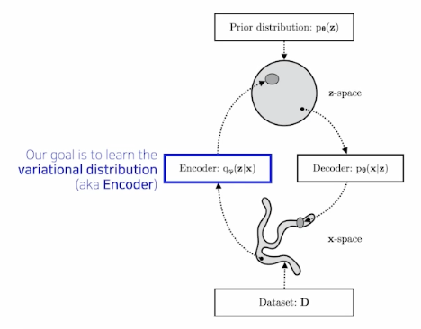
Variational Inference (VI)
- The goal of VI is to optimize the variational distribution the best matches the posterior distribution.
- Posterior distribution: \(p_\theta(z\vert x)\)
- Variational distribution: \(q_\phi(z\vert x)\)
- In particular, we want to find the variational distribution that minimizes the KL-divergence between the true posterior.
- The goal of VI is to optimize the variational distribution the best matches the posterior distribution.
MLE \[\begin{aligned} \overbrace{\log p_\theta(x)}^\text{maximum likelihood learning} &=\int_z\underbrace{q_\phi(z|x)}_{\text{For any}\;q_\phi}\log p_\theta(x)\mathrm{d}x \\&=\mathbb E_{z\sim q_\phi(z|x)}\left[\log\frac{p_\theta(x)p_\theta(z|x)}{p_\theta(z|x)}\right] \\&=\mathbb E_{z\sim q_\phi(z|x)}\left[\log\frac{p_\theta(x,z)}{p_\theta(z|x)}\right] \\&=\mathbb E_{z\sim q_\phi(z|x)}\left[\log\frac{p_\theta(x,z)q_\phi(z|x)}{p_\theta(z|x)q_\phi(z|x)}\right] \\&=\mathbb E_{z\sim q_\phi(z|x)}\left[\log\frac{p_\theta(x,z)}{q_\phi(z|x)}\right]+\mathbb E_{z\sim q_\phi(z|x)}\left[\log\frac{q_\phi(z|x)}{p_\theta(z|x)}\right] \\&=\underbrace{\mathbb E_{z\sim q_\phi(z|x)}\left[\log\frac{p_\theta(x,z)}{q_\phi(z|x)}\right]}_{\text{ELBO}\;\uparrow}+\underbrace{D_{KL}(q_\phi(z|x)\Vert p_\theta(z|x))}_{\text{Variational Gap}\;\downarrow} \end{aligned}\]
- ELBO: Evidence Lower Bound
- True posterior \(q_\phi(z\vert x)\)는 존재성은 알고 있으나 수식으로 풀어내어 계산하는 것은 불가능한 항
- 목적은 \(p_\theta\)를 \(q_\phi\)에 근사하고자 하는 것
- 이때 ELBO는 tractable quantity이므로 이를 최대화하여 variational gap을 상대적으로 줄이고자 하는 것
Evidence Lower Bound
\[\begin{aligned} \underbrace{\mathbb E_{z\sim q_\phi(z|x)}\left[\log\frac{p_\theta(x,z)}{q_\phi(z|x)}\right]}_{\text{ELBO}\;\uparrow} &=\int\log\frac{p_\theta(x|z)p(z)}{q_\phi(z|x)}q_\phi(z|x)\mathrm dz \\&=\underbrace{\mathbb E_{q_\phi(z|x)}[p_\theta(x|z)]}_\text{reconstruction term}-\underbrace{D_{KL}(q_\phi(z|x)\Vert p(z))}_\text{prior fitting term} \end{aligned}\]- Reconstruction term: encoder \(q_\phi\)와 decoder \(p_\theta\)를 모두 통과한 것으로 해석할 수 있음
- Prior fitting term — enforces the latent distribution to be similar to the prior distribution \(p(z)\).
Key Limitations
- Intractable model (hard to evaluate likelihood)
- The prior fitting term should be differentiable (\(\because\) gradient descent method), hence it is hard to use diverse latent prior distributions.
In most cases, we use an isotropic Gaussian where we have a closed-form for the prior fitting term. \[D_{KL}(q_\phi(z|x)\Vert \mathcal N(0,I))=\frac{1}{2}\sum_{i=1}^{|\mathcal D|}(\sigma_{z_i}^2+\mu_{z_i}^2-\log(\sigma_{z_i}^2)-1)\]
- Prior fitting term을 gradient descent로 최적화하기 위해서는 isotropic Gaussian을 가정할 수밖에 없기 때문에 Gaussian을 사용
- 생성된 이미지의 퀄리티로 볼 때, 추천되지 않는 방법
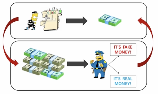
Generative Adversarial Networks
 \[\min_G\max_DV(D,G)=\mathbb E_{\mathbf x\sim p_\text{data}(\mathbf x)}[\log D(\mathbf x)]+\mathbb E_{\mathbf z\sim p_{\mathbf z}(\mathbf z)}[\log(1-D(G(\mathbf z)))]\]
GAN objective
- GAN is a two player minimax game between generator and discriminator.
Discriminator objective: \[\max_DV(G,D)=\mathbb E_{\mathbf x\sim p_\text{data}(\mathbf x)}[\log D(\mathbf x)]+\mathbb E_{\mathbf x\sim p_G(\mathbf z)}[\log(1-D(\mathbf x))]\]
The optimal discriminator is \[D_G^*(\mathbf x)=\frac{p_\text{data}(\mathbf x)}{p_\text{data}(\mathbf x)+p_G(\mathbf x)}\]
Generator objective: \[\min_GV(G,D)=\mathbb E_{\mathbf x\sim p_\text{data}}[\log D(\mathbf x)]+\mathbb E_{\mathbf x\sim p_G}[\log(1-D(\mathbf x))]\]
Plugging the optimal discriminator into the above generator objective equation we obtain \[\begin{aligned} V(G,D_G^*(\mathbf x)) &=\mathbb E_{\mathbf x\sim p_\text{data}}\left[\log \frac{p_\text{data}(\mathbf x)}{p_\text{data}(\mathbf x)+p_G(\mathbf x)}\right]+\mathbb E_{\mathbf x\sim p_G}\left[\log\frac{p_G(\mathbf x)}{p_\text{data}(\mathbf x)+p_G(\mathbf x)}\right] \\&=\mathbb E_{\mathbf x\sim p_\text{data}}\left[\log \frac{p_\text{data}(\mathbf x)}{\frac{p_\text{data}(\mathbf x)+p_G(\mathbf x)}{2}}\right]+\mathbb E_{\mathbf x\sim p_G}\left[\log\frac{p_G(\mathbf x)}{\frac{p_\text{data}(\mathbf x)+p_G(\mathbf x)}{2}}\right]-\log4 \\&=\underbrace{D_{KL}\left[p_\text{data},{\frac{p_\text{data}+p_G}{2}}\right]+D_{KL}\left[p_G,{\frac{p_\text{data}+p_G}{2}}\right]}_{2\times\text{Jenson-Shannon Divergence (JSD)}}-\log4 \\&=2D_{JSD}[p_\text{data},p_G]-\log4 \end{aligned}\]
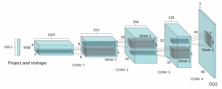
Deep Convolutional GAN
Diffusion Models
- Diffusion models progressively generate images from noise.
- 논문 이해를 위한 lecture note 링크: https://github.com/sjchoi86/2022-1-deep-learning-applications/blob/main/lecture note/08. Generative model (DDPM).pdf
- DDPM paper는 1000번의 step을 밟음. 한 이미지 생성에 몇 분씩 소요.
- 장점? 성능이 좋음. 비효율적으로 보이고 구현하기는 더더욱 어려우나, 월등히 좋은 성능.
- Autoregressive model 성능도 좋다는 것이 알려지면서 2022년 기준 엎치락뒤치락하는 상황.
Diffusion Models
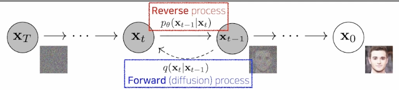
Forward (diffusion) process progressively injects noise to an image. \[p_\theta(\mathbf x_{t-1}|\mathbf x_t):=\mathcal N(\mathbf x_{t-1};\mu_\theta(\mathbf x_t,t),\Sigma_\theta(\mathbf x_t,t))\]
- The reverse process is learned in such a way to denoise the perturbed image back to a clean image.
- DDPM 간단 요약: 굉장히 오랜 스텝을 거쳐 noise vector를 original image로 개선해나가는 과정
DALL-E 2
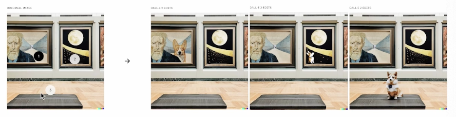
- 이미지의 특정 부분을 editing 할 수 있다는 점이 인상적